Purrception 🐈: A Hybrid Approach to Image Generation

Published Apr 5, 2026 · 20 min read · Last updated Apr 16, 2026

Introduction

Generative modeling in a few words

In the generative modeling task, the goal is to create new, realistic data that resembles a set of examples already seen before. For instance, if we show to an AI model thousands of pictures of cats, we want it to learn the underlying patterns and structures well enough to be able to generate new images of cats that have never existed before.

Most commonly, this is done through probabilistic modeling. Formally, we assume the data comes from a probability distribution $p_{\text{data}}$ (unknown to the model). Given a finite number of samples drawn from that distribution, $\mathcal{D} = \{x_1, x_2, \dots, x_N\} \subseteq \mathbb{R}^D$, the model is trying to approximate it by learning the parametrized probability distribution $p_{\theta}$.

Going from noise to images

Flow models

For image generation, most recent approaches aim to solve this task by mapping noise to data, i.e., learning a time-dependent mapping between a simple noise distribution $p_0$ from which it is easy to sample from (e.g., a Gaussian or uniform distribution) to the more complicated target data distribution $p_1$.

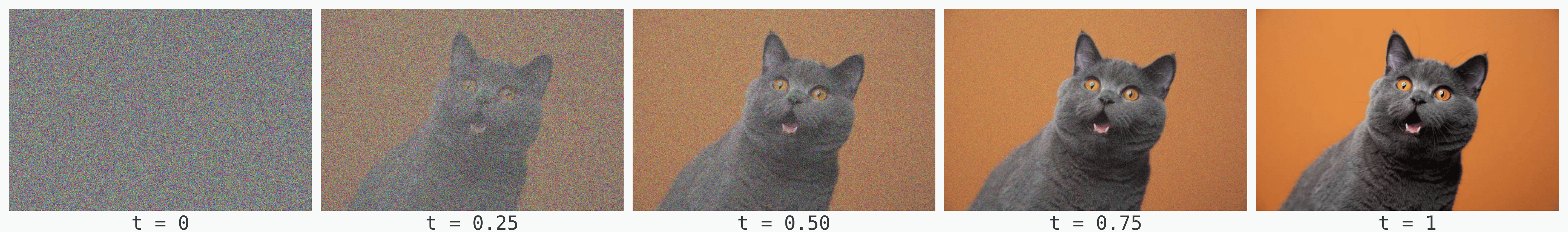
What these models do is instead of learning the distribution of interest directly, they use a distribution from which they can sample from easily and then map the samples to a target distribution. This approach of learning a data distribution from noise is embodied (broadly speaking) by flow models.

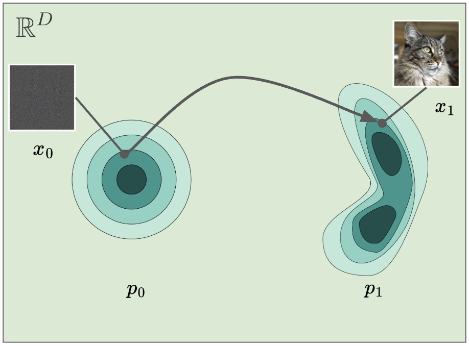
A flow is characterized by two things:

• a starting point $x_0 \in \mathbb{R}^D$ and
• a time-dependent diffeomorphismA diffeomorphism between open sets in $\mathbb{R}^D$ (more generally, smooth manifolds) is a bijection $f: U \to V$ such that $f$ and $f^{-1}$ are both smooth (infinitely differentiable). Equivalently, $f$ is smooth, invertible, and its Jacobian determinant is nowhere zero, so $f^{-1}$ is smooth by the inverse function theorem. Intuitively: a reshaping that can be undone smoothly, with no folding or tearing.For more detail, the Wikipedia article on diffeomorphisms is a strong formal and complete reference. $\psi_t: [0,1] \times \mathbb{R}^D \rightarrow \mathbb{R}^D$, where $x_t = \psi_t(x_0),\forall t \in [0,1 ]$.

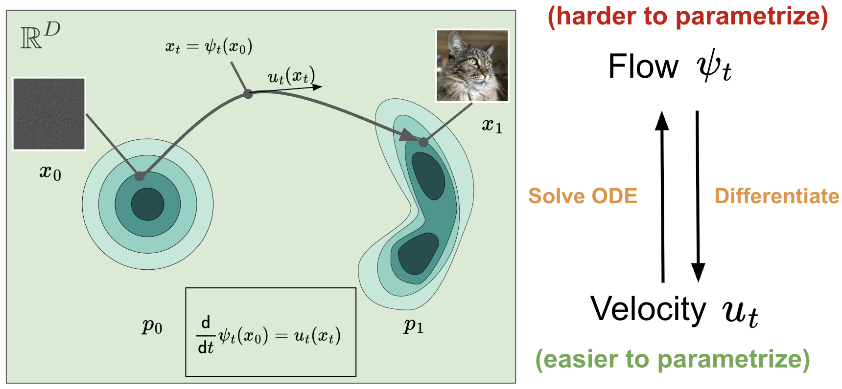
The goal is to learn a flow such that for every $x_0 \sim p_0$, we have $x_1 = \psi_1(x_0)$, where $x_1 \sim p_1$. However, learning a flow directly can be challenging because you need to make sure all mathematical properties of a diffeomorphism are met. For example, a flow $\psi_t$ must be invertible at all times $t$ and ensuring a neural network always remains invertible is extremely challenging. In simple terms, it is hard to parametrize!

What a flow model does is obtain the flow indirectly by learning a time-dependent vector field $u_t(x_t)$: instead of learning the entire path at once, we learn, at each time and position, the local direction in which state should move.

Not every formulation builds that field in the same way. In continuous normalizing flows (CNFs), $u_t$ is what you learn directly—the network outputs a velocity field, and training shapes it so that transporting the base distribution $p_0$ along that field recovers the data distribution $p_1$ (through the continuity equation and related objectives). Flow matching, which we discuss next, flips the emphasis: you first fix how noise and data should be linked (most often by interpolating between a sample $x_0 \sim p_0$ and a sample $x_1$ from the data, which pins down a target velocity along that path) and the model then regresses to that already-specified $u_t$ rather than discovering the field from scratch.

Either way, velocity and position stay tied together by a one-to-one relationship described by an Ordinary Differential Equation (ODE):

Luckily, we can simulate the solution of the ODE quite easily using numerical methods. This means that, in order to generate new samples, one needs to:

• sample $x_0 \sim p_0$ and then
• simulate the solution of an ODE via a numerical method solver to get $x_1 \sim p_1$.

Flow Matching

One scalable method for learning flow models is Flow Matching (FM) [1]. This approach gained a lot of popularity and it is extensively used nowadays in text-to-image generation (e.g., Stable Diffusion 3 [2]), text-to-video generation (e.g., MovieGen from Meta [3]), or robot control via Vision-Language-Action models [4].

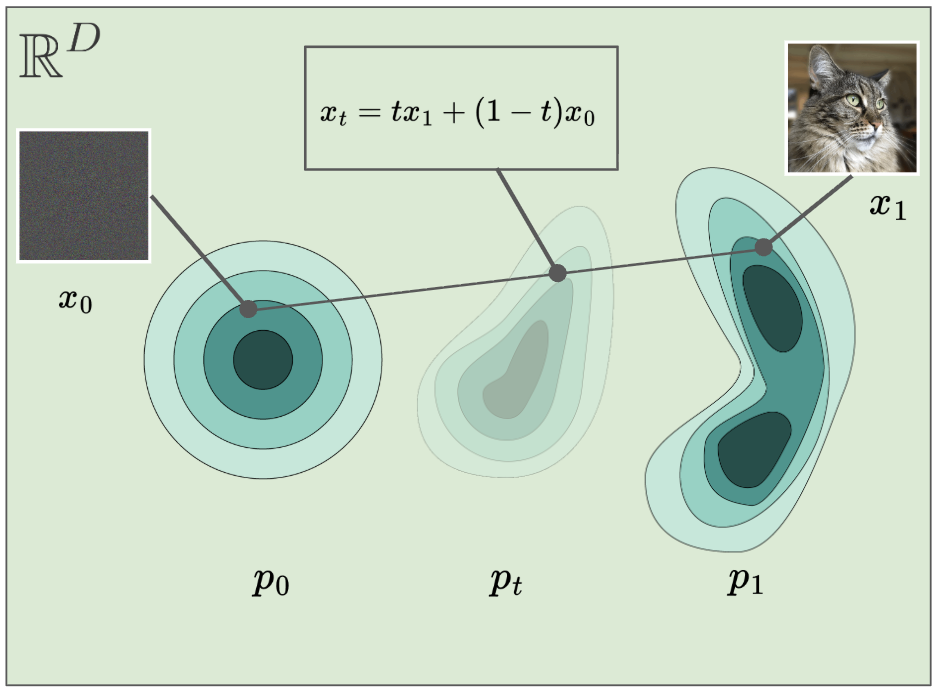
In Flow Matching, learning the velocity field is treated as a regression task and one training step can be summarized below:

• Sample $x_0 \sim p_0$
• Sample $x_1 \sim \mathcal{D}$
• Sample $t \sim \mathcal{U}(0,1)$
• Calculate the point $x_t = (1 - t)x_0 + tx_1$ on the straight path between $x_0$ and $x_1$.
• Compute the velocity $u_t^{\theta}(x_t)$
• Compute the loss $\mathcal{L}(\theta) = \left\lVert u_t^{\theta}(x_t) - (x_1 - x_0)\right\rVert_2^2$. For this straight-line interpolation, the target velocity is the constant vector from $x_0$ to $x_1$, since $\frac{\mathrm{d}x_t}{\mathrm{d}t} = x_1 - x_0$.
• Update the model parameters $\theta$.

where $u_t^{\theta}(x_t)$ is a neural network that receives as input the timestep $t$ and the interpolant $x_t$.

That’s it! By doing this for multiple steps with multiple data samples $x_1$, noise samples $x_0$, and timesteps $t$, the neural network eventually ends up learning a comprehensive vector field $u_t$ that works for the entire space.

The Need of a Latent Space

An image is usually high-dimensional. For instance, if we talk about a squared RGB image of $1024 \times 1024$ resolution, then our generative model would need to learn the joint distribution of more than 3 million pixels! This means that the training and generation can be quite expensive and, in many cases, learning such joint distribution is even an intractable problem.

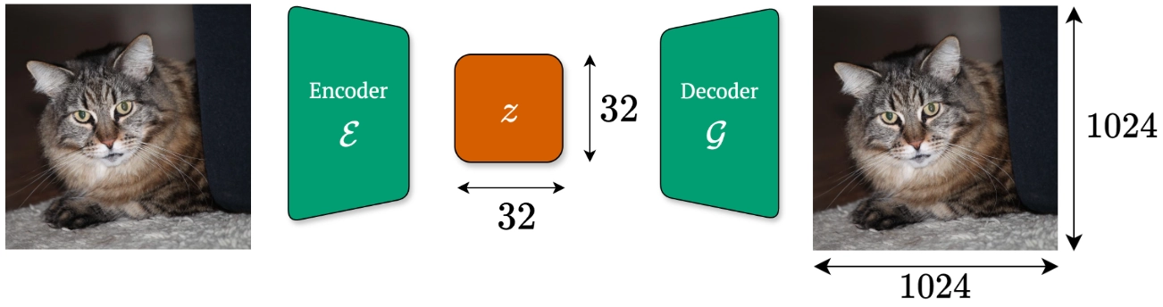
Most recent approaches in image generation employ a latent space, where the images are brought to compressed, lower-dimensional representations $z \in \mathbb{R}^d, d < D,$ via an autoencoder. An autoencoder consists mainly of two components:

• an encoder $\mathcal{E}:\mathbb{R}^D \rightarrow \mathbb{R}^d$ that maps an image $x$ to the latent representation $z = \mathcal{E}(x)$, and
• a decoder $\mathcal{G}:\mathbb{R}^d \rightarrow \mathbb{R}^D$ that maps the latent representation $z$ back to the pixel space $\bar{x} = \mathcal{G}(z)$

where $\bar{x}$ is a high-fidelity approximation of $x$.

The core idea is that instead of learning a flow model to map noise directly to images, the flow model now maps noise to the latent representations, which are further passed through the decoder $\mathcal{G}$ to get the final image. Easy, right? We recommend reading Dieleman’s blog post [5] on generative modeling in latent space, where he discusses how autoencoders are pre-trained and how common generative techniques are used in latent space.

Vector-Quantized Latent Spaces

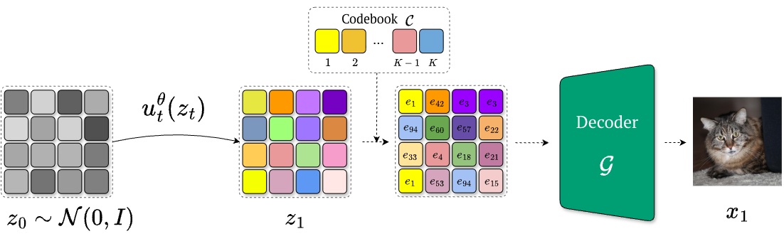
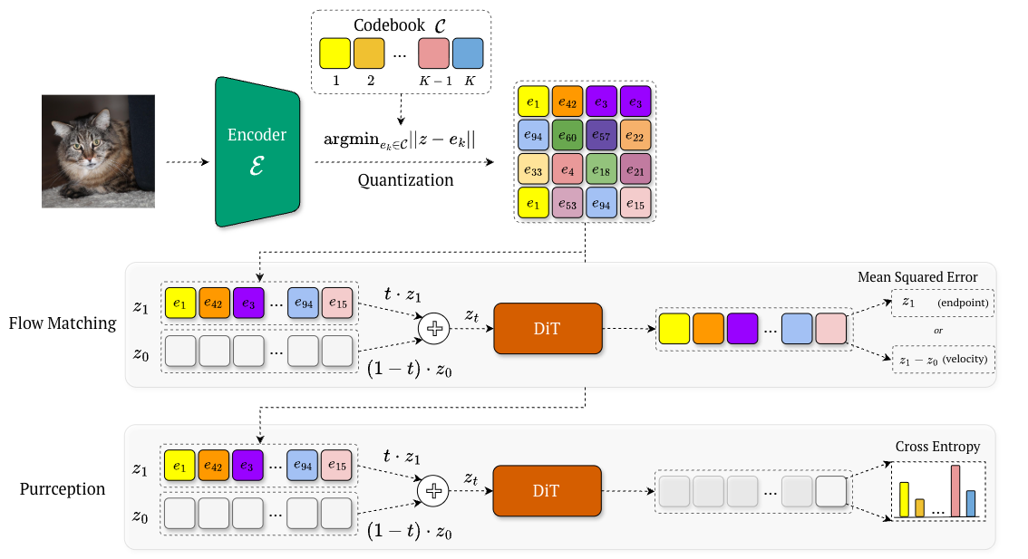
In this blogpost, we will focus on vector-quantized (VQ) latent spaces and how the latent representations are stored. In addition to the encoder $\mathcal{E}$ and the decoder $\mathcal{G}$, VQ autoencoders (e.g., VQ-VAE [6], VQ-GAN [7]) use a finite set of vectors $\mathcal{C} = \{e_k\}_{k=1}^K \subseteq \mathbb{R}^d$ popularly called a codebook. Given an image $x \in \mathbb{R}^D$, the encoder output is quantized to its nearest codebook vector in $\mathcal{C}$, namely:

Equivalently, one can only store the index:

We can see that the latent representation can be at once a discrete code index and a continuous embedding. Existing generative methods either operate in the continuous embedding space (while ignoring the categorical structure), or modeling indices directly (while discarding geometric information).

This limitation motivates the need for a hybrid approach that can operate in the continuous embedding space while learning is driven by the cross-entropy over codebook indices.

Purrception

To understand better the current modeling problem in a VQ latent space, let’s visualize how a fully continuous and a fully discrete flow model operate in this latent space.

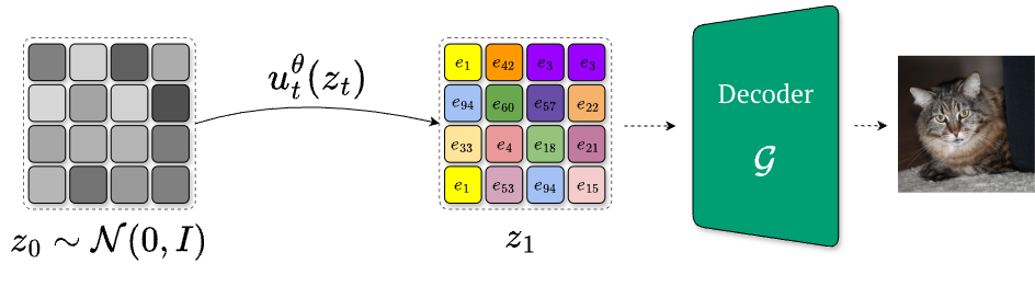
Continuous flow models (such as latent diffusion [10] and flow matching [1]) operate in $\mathbb{R}^d$, treating codebook vectors as continuous. Geometry is preserved, but discreteness is lost because the model never receives the categorical learning signal suitable for this latent space, cannot express uncertainty over multiple plausible codes, and has no logits from which to derive control, such as temperature scaling.

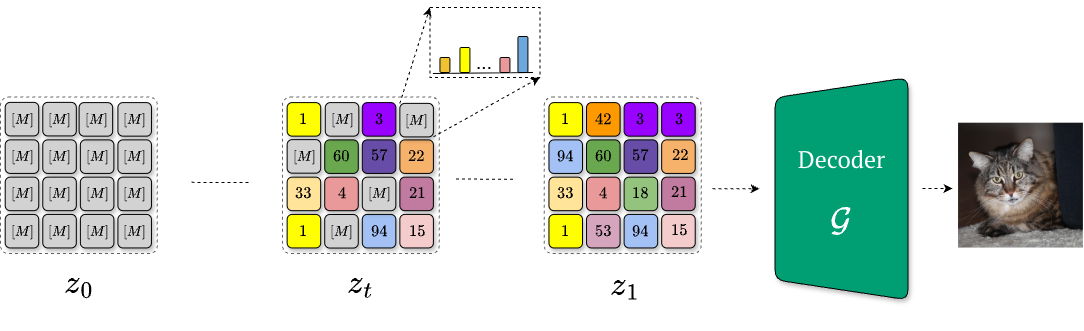
Fully discrete flow models instead predict categorical indices directly. This restores categorical supervision, but once everything is reduced to indices, semantically nearby codes are no longer geometrically nearby. For instance, discrete flow matching [12] learns how to denoise progressively a fully-masked tensor $z_0$ (i.e., via a time-dependent scheduler) in order to obtain the final, quantized latent representation $z_1$. While this aligns with the quantized structure, it collapses geometry: once reduced to raw indices, semantically related codes are treated as unrelated tokens. Consequently, the final predictions degenerate into discrete “teleports” between indices, eliminating interpolation and making both uncertainty modeling and temperature scaling meaningless.

An ideal solution would combine the strenghts of both worlds: exploit the smooth geometry of embeddings and provide categorical supervision over indices. This is what variational flow matching [8] can do and we will focus our attention further on how it works.

Theoretical View: What Is Variational Flow Matching and How Does It Work?

First, let’s take some steps back and dive deeper into the math behind flow matching.

We have already seen that we can learn the velocity field (and thus the flow) via an ODE. This is equivalent to learning a velocity field that satisfies the continuity equation, also known as the continuous normalizing flows:

where $p_t$ is the probability path at time $t$, generated by the velocity field $u_t$.

Flow matching starts from observing that, given a choice of interpolation between noise and data (e.g., linear, where $x_t = (1 - t)x_0 + tx_1$), we can derive a conditional velocity field $u_t(x \mid x_1)$ that satisfies the continuity equation towards (i.e., conditioned on) a specific point.

A corresponding velocity field $u_t(x)$ which satisfies the continuity equation for the (marginal) probability path $p_t(x)$, can be further expressed in terms of an (intractable) expectation with respect to its posterior $p_t(x_1 \mid x)$, namely:

A flow matching algorithm is to learn the velocity field $u_t^{\theta}(x)$ that approximates $u_t(x)$ via a regression task:

which can be tractable by optimizing the conditional flow matching objective:

These two objectives have the same gradients w.r.t. $\theta$ (and thus learn the same thing!), as proved in the original Flow Matching paper.

On the other hand, variational flow matching treats flow matching as a variational inference problem. This essentially means that now the goal is to approximate the posterior distribution $p_t(x_1 \mid x)$ with another (learnable) distribution $q_t^{\theta}(x_1 \mid x)$ (often called a variational posterior).

To do that, we need a metric that can assess how similar (or different) two distributions are. One popular metric is the Kullback-Leibler (KL) divergence (also called the relative entropy), which measures how much an approximating distribution $Q$ is different from a true distribution $P$.

For our use case, if we want to approximate $p_t(x_1 \mid x)$ with $q_t^{\theta}(x_1 \mid x)$, we need to minimize the expectation over $t$ of the KL divergence between the joint distributions $p_t(x_1, x) = \frac{p_t(x)p_t(x_1 \mid x)}{p_t(x_1)}$ and $q_t^{\theta}(x_1, x) := \frac{p_t(x)q_t^{\theta}(x_1 \mid x)}{p_t(x_1)}$ .

where $C$ is a constant that does not depend on the parameters $\theta$.

The resulting learning velocity field would thus be given by:

where $\mu_t^{\theta}(x) := \mathbb{E}_{q_t^{\theta}}[x_1 \mid x]$ and the conditional field is the linear (or optimal transport) interpolation. Though this objective initially looks intractable, the authors show that the task of learning the variational approximation only needs to be learned dimension-wise in the mean, because $\mathbb{E}_{q_t^{\theta}}[x_1^d \mid x]$ only depends on the marginal $q_t^{\theta}(x^d \mid x)$ — an approach called mean-field variational flow matching.

What is nice about variational flow matching is its flexibility in choosing the variational distribution $q_t^{\theta}$, which makes it a general framework for different domains, including Riemannian geometries, molecules, graphs, physical and biological systems, tabular data, as well as simulation-based inference.

Variational Flow Matching in Vector Quantized Latent Space

In the context of vector-quantized image generation, it is worth noting that the each endpoint must be one of the finite codebook $\mathcal{C}$ embeddings, meaning that the posterior is categorical over the discrete latent codes. That is, our variational posterior should be given by:

where $\pi_t^{\theta}(z_t)$ is the probability distribution over the codebook vectors outputted by a neural network (for example, a Diffusion Transformer [9]). Conditioning this posterior on the noisy $z_t$ yields a distribution over discrete indices while still defining a mapping in the continuous embedding space, as we can compute:

where $\mu_t(z_t) := \sum_{k=1}^K\pi_t^{\theta,k}(z_t) \cdot e_k$ and $\pi_t^{\theta, k}(z_t)$ is the probability to have as endpoint the codebook vector $e_k$.

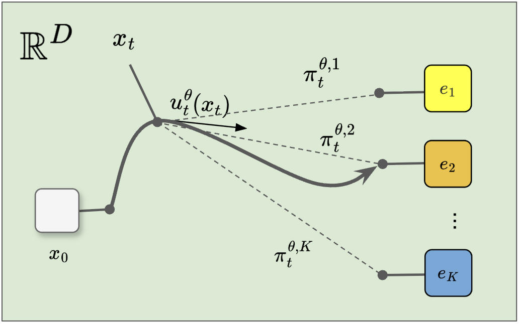
This ensures that the uncertainty over multiple plausible codes is translated into smooth, geometry-aware motion, rather than discrete “teleports” between unrelated indices.

Training follows from the Variational Flow Matching objective, which in this case reduces to the cross-entropy loss between the predicted posterior and the ground-truth code indices:

where $x \sim \mathcal{D}$ is sampled from the data, $z_1$ and $c$ are the corresponding quantized image and latent code, respectively, and $z_t$ is simply a time-dependent linear interpolation between $z_0$ and $z_1$.

Compared to Flow Matching, Purrception is trained similarly, the only difference being that Flow Matching predicts the velocity field or the endpoint via Mean-Squared Error, whereas Purrception employs a Cross-Entropy loss!

Results and Discussion

We validate the performance of Purrception through a series of experiments. In our experiments, we evaluate on ImageNet on 256x256 resolution, using both the Stable Diffusion’s [10] and LlamaGen’s [11] tokenizers (kept frozen during training). We employ a Diffusion Transformer (DiT) [9] architecture for training the flow model.

Convergence speed

First, we perform a comparative study between Purrception, continuous flow matching (CFM) and discrete flow matching (DFM) [12]. For continuous flow matching, we consider two objectives: the classical regression task of predicting the velocity field (denoted simply as CFM) and the task of predicting the endpoint (denoted as CFM-endpoint), allowing us to measure the effects of both (1) switching to endpoint prediction, and (2) using our discrete objective compared to the continuous baseline. For a fair comparison, we used the same training configurations, and we sample all images using Euler with 100 integration steps as ODE solver.

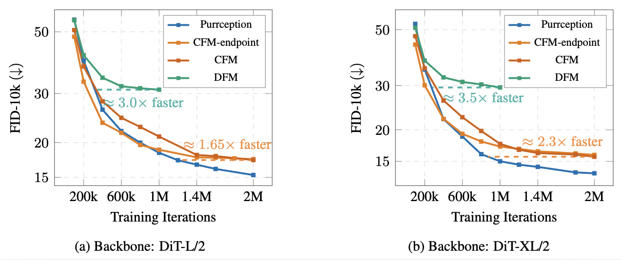
We show that Purrception converges faster (i.e., in fewer training iterations) to a low FID. These results underscore the advantage of Purrception’s hybrid formulation. By receiving direct categorical supervision (unlike CFM), the model learns discrete structure more efficiently, while its use of continuous embedding space (unlike DFM) enables smooth geometry-aware transport rather than slow, discrete jumps. This combination accelerates optimization, leading to both faster convergence and stronger sample quality

Optimizing sample quality via softmax temperature scaling

Temperature scaling is a long-standing technique in language modeling, used to balance coherence and diversity during sampling. In the context of VQ image synthesis, continuous flow methods (e.g., CFM) cannot exploit this mechanism at all, since they lack categorical logits. Fully discrete models (e.g., DFM) can in principle apply temperature scaling to their logits, but because they commit to hard index selections at each step, adjusting $\tau$ has little practical effect – the sampling collapses to discrete jumps regardless of the distribution’s softness. In contrast, Purrception retains uncertainty in the logits while transporting through the continuous embedding space, which means temperature scaling can be naturally used.

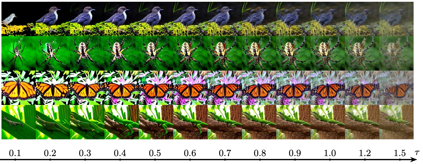
To test the effect of the softmax temperature during inference, we conduct an ablation study with a DiT-XL/2 backbone trained for one million iterations. During training, we keep $\tau$ to the default 1.0, varying the temperature only at inference.

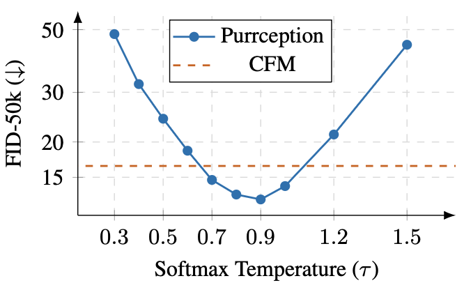
In our experiments, we observe a clear U-shaped curve: performance improves as $\tau$ increases from very low values, reaches an optimum around $\tau \approx 0.8-0.9$ and then degrades as $\tau$ becomes larger. Qualitatively, low $\tau$ values produce overly deterministic and simplistic images, while high $\tau$ values lead to noisy and incoherent generations.

These findings highlight two things:

• even though Purrception has been trained with a constant $\tau = 1.0$, the data distribution is best approximated for lower softmax temperatures;
• adjusting $\tau$ is a simple, training-free approach to improve the sample quality.

Future work could consist of developing principled softmax temperature schedules during inference or varying $\tau$ during training.

Quantitative results

To test how well Purrception performs against similar methods, we train Purrception at scale for 3.5M iterations with a DiT-XL/2 backbone.

The table below highlights a comparison with popular image generation methods, similar to Purrception in model size and methodology, including autoregressive methods, discrete diffusion and masked generative models, as well as continuous diffusion models. Purrception is competitive in FID score. Notably, Purrception outperforms all discrete diffusion and masked generative models. It also shows stronger performance against most autoregressive methods while having less parameters and/or benefiting from natively faster decoding than large-token autoregressive models (which often rely on inference optimizers).

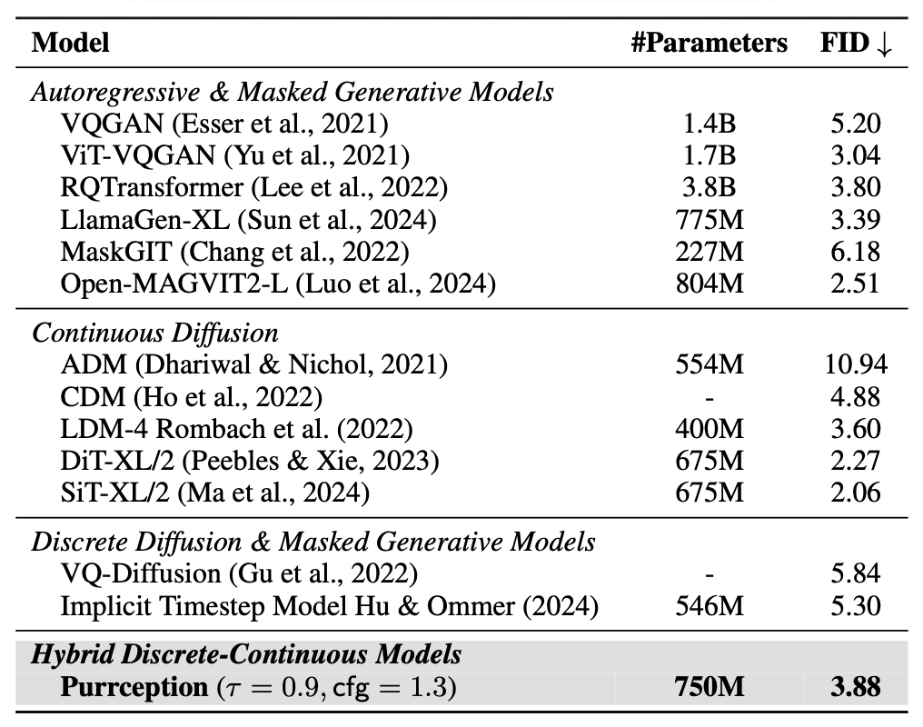
Against strong continuous diffusion baselines, Purrception falls short on important baselines like DiT-XL/2 and SiT-XL/2 baselines. We believe this is mainly due to two reasons:

• the use of high-quality VAE autoencoders in those models, which are known to produce lower FID scores than VQ tokenizers at equivalent scales;
• their considerably longer training schedules (twice as many iterations as used for Purrception).

Despite this gap, Purrception’s strong results highlight that our hybrid design can approach the performance of top-tier diffusion models, positioning it as a promising direction for future generative modeling.

Conclusion

We introduced Purrception, an adaptation of Variational Flow Matching to VQ image generation. This method is a hybrid in the sense that it retains continuous transport in the embedding space while supervising with a categorical posterior over codebook indices.

This design addresses the core trade-off of existing approaches: unlike CFM, Purrception benefits from categorical supervision, and unlike DFM, it avoids collapsing geometry into hard index jumps. The result is a model that learns, broadly speaking, what to choose and where to go, expressing uncertainty over plausible codes in a geometry-aware way.

Empirically, Purrception outperforms both CFM and DFM on ImageNet-1k 256 × 256 benchmark, converging faster and achieving superior FID while preserving the efficiency of flow matching. Further ablations confirm that logits provide a controllable quality knob through softmax temperature scaling.

Limitations and Future Work

Our approach is currently limited by its reliance on a fixed, pretrained VQ autoencoder, which makes performance dependent on the initial tokenization quality. While the model is competitive on 256 × 256 ImageNet-1k, its generalization to other datasets or higher resolutions needs validation, and it does not yet match the performance of top-tier continuous diffusion models.

Future work could directly address these limitations by exploring different VQ models or jointly training the autoencoder with the flow model. Broader research directions include extending this hybrid perspective to domains like audio, video, and 3D shapes, as well as developing principled temperature schedules and a stronger theory for categorical objectives. Finally, because the model remains a continuous flow, it supports distillation into highly efficient, few-step samplers and can incorporate guidance, paving the way for practical generative pipelines.

References

[1] Lipman, Y., Chen, R. T. Q., Ben-Hamu, H., Nickel, M., & Le, M. (2022). Flow Matching for Generative Modeling. arXiv:2210.02747.

[2] Esser, P., Kulal, S., Blattmann, A., Entezari, R., Müller, J., Saini, H., Levi, Y., Lorenz, D., Sauer, A., Boesel, F., Podell, D., Dockhorn, T., English, Z., Lacey, K., Goodwin, A., Marek, Y., & Rombach, R. (2024). Scaling Rectified Flow Transformers for High-Resolution Image Synthesis. arXiv:2403.03206.

[3] Polyak, A., Zohar, A., Brown, A., Tjandra, A., Sinha, A., Lee, A., Vyas, A., Shi, B., Ma, C.-Y., Chuang, C.-Y., Yan, D., Choudhary, D., Wang, D., Sethi, G., Pang, G., Ma, H., Misra, I., Hou, J., Wang, J., Jagadeesh, K., Li, K., Zhang, L., Singh, M., Williamson, M., Le, M., Yu, M., Singh, M. K., Zhang, P., Vajda, P., Duval, Q., Girdhar, R., Sumbaly, R., Rambhatla, S. S., Tsai, S., Azadi, S., Datta, S., Chen, S., Bell, S., Ramaswamy, S., Sheynin, S., Bhattacharya, S., Motwani, S., Xu, T., Li, T., Hou, T., Hsu, W.-N., Yin, X., Dai, X., Taigman, Y., Luo, Y., Liu, Y.-C., Wu, Y.-C., Zhao, Y., Kirstain, Y., He, Z., He, Z., Pumarola, A., Thabet, A., Sanakoyeu, A., Mallya, A., Guo, B., Araya, B., Kerr, B., Wood, C., Liu, C., Peng, C., Vengertsev, D., Schonfeld, E., Blanchard, E., Juefei-Xu, F., Nord, F., Liang, J., Hoffman, J., Kohler, J., Fire, K., Sivakumar, K., Chen, L., Yu, L., Gao, L., Georgopoulos, M., Moritz, R., Sampson, S. K., Li, S., Parmeggiani, S., Fine, S., Fowler, T., Petrovic, V., & Du, Y. (2024). Movie Gen: A Cast of Media Foundation Models. arXiv:2410.13720.

[4] Black, K., Brown, N., Driess, D., Esmail, A., Equi, M., Finn, C., Fusai, N., Groom, L., Hausman, K., Ichter, B., Jakubczak, S., Jones, T., Ke, L., Levine, S., Li-Bell, A., Mothukuri, M., Nair, S., Pertsch, K., Shi, L. X., Tanner, J., Vuong, Q., Walling, A., Wang, H., & Zhilinsky, U. (2024). $\pi_0$: A Vision-Language-Action Flow Model for General Robot Control. arXiv:2410.24164.

[5] Dieleman, S. (2025). Generative modelling in latent space. Blog post. https://sander.ai/2025/04/15/latents.html

[6] van den Oord, A., Vinyals, O., & Kavukcuoglu, K. (2017). Neural Discrete Representation Learning. NeurIPS 2017. arXiv:1711.00937.

[7] Esser, P., Rombach, R., & Ommer, B. (2021). Taming Transformers for High-Resolution Image Synthesis. CVPR 2021. arXiv:2012.09841.

[8] Eijkelboom, F., Bartosh, G., Naesseth, C. A., Welling, M., & van de Meent, J.-W. (2024). Variational Flow Matching for Graph Generation. NeurIPS 2024. arXiv:2406.04843.

[9] Peebles, W., & Xie, S. (2022). Scalable Diffusion Models with Transformers (DiT). arXiv:2212.09748.

[10] Rombach, R., Blattmann, A., Lorenz, D., Esser, P., & Ommer, B. (2022). High-Resolution Image Synthesis with Latent Diffusion Models. arXiv:2112.10752.

[11] Sun, P., Jiang, Y., Chen, S., Zhang, S., Peng, B., Luo, P., & Yuan, Z. (2024). Autoregressive Model Beats Diffusion: Llama for Scalable Image Generation (LlamaGen). arXiv:2406.06525.

[12] Gat, I., Remez, T., Shaul, N., Kreuk, F., Chen, R. T. Q., Synnaeve, G., Adi, Y., & Lipman, Y. (2024). Discrete Flow Matching. NeurIPS 2024. arXiv:2407.15595.